AI-era DC Interconnect: Beyond Single Chips, Competing as a Network — Is There a China Play?

Under the scaling laws of AI foundation models, parameter counts keep ballooning and multi-turn context must be retained for longer. Single-card compute and on-card memory can no longer sustain state-of-the-art training and inference, so AI workloads must run on ultra-large clusters composed of massive xPUs working in concert.

What stitches single cards into a cluster and thousands of heterogeneous chips inside and across clusters into a machine that works as one is the AI interconnect network.

Recent roadmaps from GPGPU and AI ASIC vendors show the focus has shifted from peak single-die FLOPS to the engineering of large-scale clusters.

Today, training is sharded across tens of thousands of xPUs. Each iteration and gradient step involves heavy collective communication among xPUs; under synchronous parallelism, every card must wait for the slowest link before moving on (the bottleneck effect).

In the single-die era, Chinese vendors lagged far behind. In the AI interconnect era, where high bandwidth and low latency are paramount, Jensen Huang has said that single-die weaknesses can be offset by interconnect, which happens to be Huawei’s strength — a custom UB protocol, its own switches, and powerful interconnect capability.

Dolphin Research will unpack the hierarchy of AI interconnects through a series of notes. This piece starts from the basics:

1) What does connectivity look like in an AI data center?

2) What are the key concepts and building blocks?

I. What is network connectivity?

Building a data center requires GPUs, CPUs and other xPUs, storage, NICs, switches, and more. Connectivity links these devices over fiber and copper to form a high-speed fabric for information exchange.

The core elements are not fundamentally different from traditional networks. But tighter coupling at higher speed and bandwidth raises the engineering bar.

Let’s first look at the AI network hierarchy used by $NVIDIA(NVDA.US) &$AMD(AMD.US), which is broadly representative. By physical scope from inside out, it can be split into three layers:

1) Within a compute tray — CPU to surrounding devices;

2) Within a rack and across trays in the rack — xPU-to-xPU;

3) Data center to data center. See below:

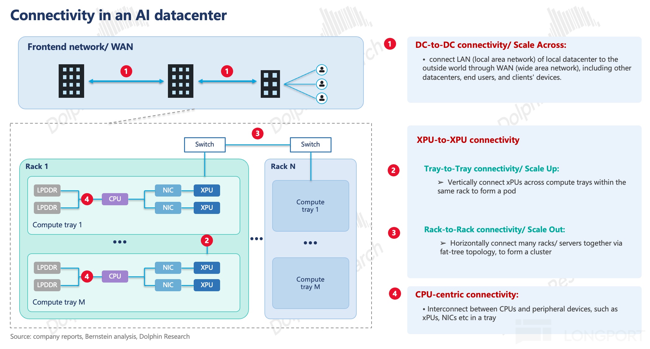
Think of an AIDC as a campus built to deliver a mega project (AI workloads). The campus has many office buildings (racks), each with multiple compute floors (compute trays) and dispatch floors (switch trays with proprietary switch ASICs for traffic fan-out and in-network compute).

The core roles are project managers (CPUs) who assign tasks, fetch data, and interface externally, and engineers (xPUs) who do the heavy lifting, with a front desk (NIC) for external I/O. The project is split into tens of thousands of parallel tasks, and 'who talks to whom and how fast they align' determines the overall schedule.

1) Within the same tray — CPU-to-peripheral interconnect: this layer coordinates traffic among CPUs, xPUs, NICs and other peripherals. Physically it is PCB traces measured in centimeters with ultra-low latency in nanoseconds. Functionally, it handles internal/external data movement and dispatches work to xPUs.

2) Intra-/inter-rack — xPU-to-xPU interconnect: this is the compute brain of the AI era, i.e., the engineers doing the work. Given extreme AI compute demands, the engineers must be tightly linked to act like one super engineer, making this the fastest-evolving layer and the focus of this note.

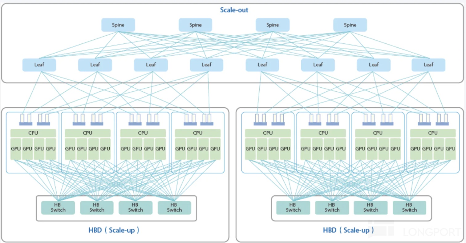
- Tray-to-tray (Scale-up): a single office floor hosts multiple engineers. Even if they are close, they do not talk peer-to-peer; instead each sends information to the dispatch floor (switch tray), which forwards centrally.

The reason: communication is not pairwise but many-to-many among dozens or hundreds. If people had to pass messages down the line, relays would add delay. By sharing all messages with the dispatcher (switch), which then delivers directly to the destination, we avoid relay latency. In other words, even though GPUs on a tray sit close, they are not directly wired to each other.

Physically, traffic leaves the xPU via PCB off the tray, then runs over copper into the switch tier. As xPU counts grow, this link keeps evolving. Today it is primarily copper, whose physics sets the limits of engineer–dispatcher–engineer communication.

Note: labeling Scale-Up/Out by physical distance (in-/out-of-rack) is imprecise but intuitive. We will see Nvidia Rubin Ultra extending the Scale-Up domain beyond a rack. The true difference lies in protocol semantics:

- Scale-Up is like direct load/store. With an address, the switch ASIC fetches by address (memory semantics with direct addressed R/W), yielding lower latency;

- Scale-Out is like parcel delivery. Content must be encapsulated and addressed, then forwarded and acknowledged (message semantics requiring protocol encapsulation and confirmation).

By communication semantics, in common topologies (excluding Huawei), the Scale-Up domain typically includes only xPUs, while other in-rack components (CPUs, storage, etc.) sit outside the domain.

Take CPUs: if a CPU needs to reach a CPU on another tray, it uses message semantics over the same path as one server talking to another: CPU → PCIe → NIC/DPU → switch → peer DPU → PCIe → CPU. That is effectively Scale-Out even within the same rack.

- Rack-to-rack (Scale-out): multiple buildings (racks) are chained into a coordinated training cluster (Pod/SuperPod). Cross-building traffic no longer goes through the dispatch floor (switch tray) but is handed from xPU to NIC.

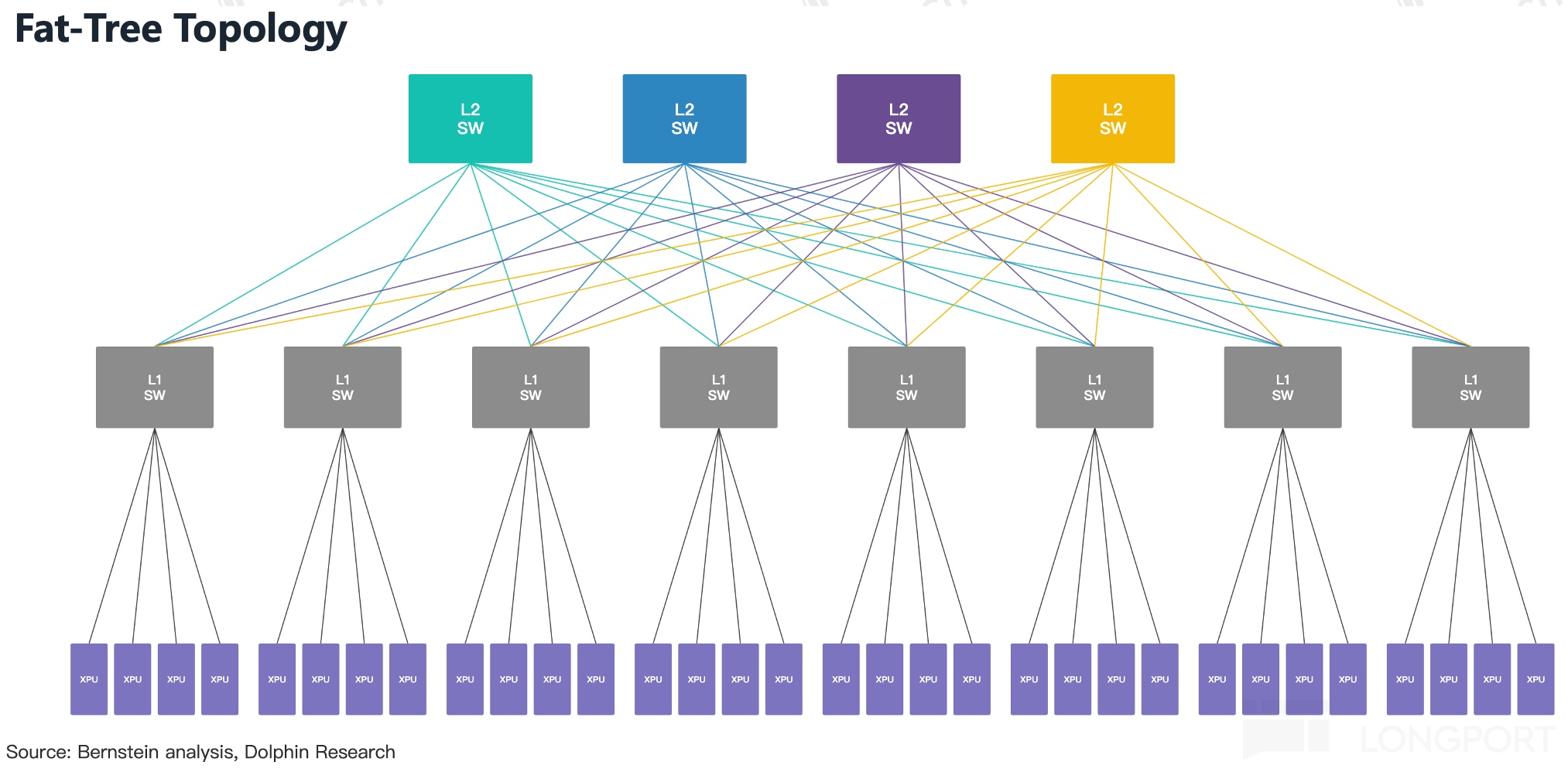
It then traverses Ethernet switches (think campus mail room), relying on 400G/800G/1.6T optics and using two-/three-tier fat-tree topologies (see below). The challenge shifts from raw speed to congestion control, cost efficiency, and orchestrating tens of thousands of accelerators.

3) Data center interconnect (Scale-across): long-haul optical networks link multiple campuses or regions, enabling cross-region workload distribution, data replication, and end-user access, relying on coherent DWDM optics. Reach spans tens to hundreds of kilometers, with per-wavelength bandwidth from 400G to 800G and moving toward 1.6T/3.2T. Because it carries inter-region traffic rather than synchronous training flows, higher latency is acceptable.

II. Network connectivity: key hardware and how it works

The above describes 'who talks to whom.' Next is how they talk. The stack boils down to two categories:

a) Hardware: PCBs, switches, NICs, optics, copper cables, fiber, etc.;

b) Software: interconnect protocols — ultimately an ecosystem contest where whoever sets the standards ships more hardware and wins more designs.

We start with hardware:

1) Hardware: shipments and share by protocol define the hard power of an interconnect ecosystem

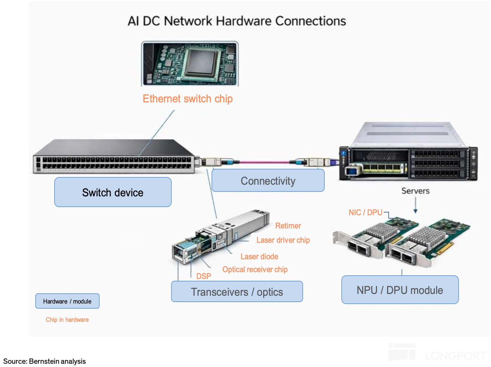
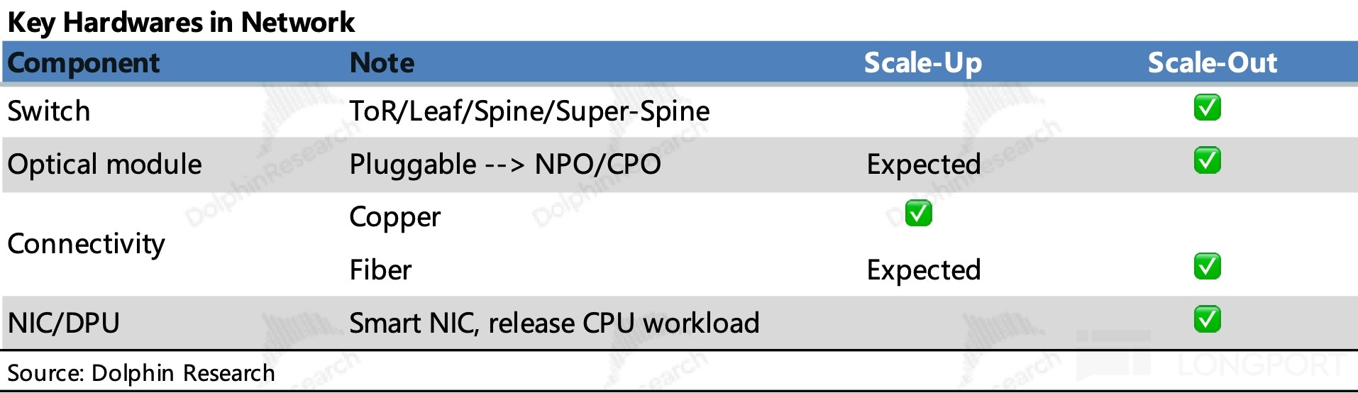
Hardware falls into three module classes: switches, optical/connection components, and NIC/DPU. Each centers on dedicated chips that deliver bandwidth, signal integrity, and offload compute for AI clusters.

a) Switches: high value-add, high GPM

Switches build the network and are the core aggregation/forwarding nodes in AIDC, scheduling traffic among xPUs — the campus mail room in our analogy. The switch ASIC determines system throughput, latency, and power.

Aggregate bandwidth is a function of port count and per-port rate. Mainstream boxes support 51.2T today and are moving to 102.4T, with 400G/800G/1.6T port rates.

In fat-tree designs, switches tier into ToR/Leaf, Spine, and Super-Spine at three-tier scale. ToR/Leaf sit atop the rack and connect down to server NICs, the only tier directly attached to xPUs, while upper tiers interconnect switches and fan out from Spine to Super-Spine as layers grow.

b) Optics/connectivity

• Optical: high chip value-add, high GPM; module value-add high but competitive

Optical modules bridge switch ASICs/NICs and links via bidirectional E/O & O/E conversion, acting as the 'translator' in data transport. They are indispensable in Scale-Out and increasingly extend Scale-Up beyond copper’s reach.

As link rates move to 800G/1.6T and even 3.2T, power, thermal, and signal integrity become bottlenecks, pushing architectures from pluggables (mainly 400G/800G) toward LPO and CPO. For details see 技术演进 and 产业链梳理.

• Media: mid value-add, highly competitive

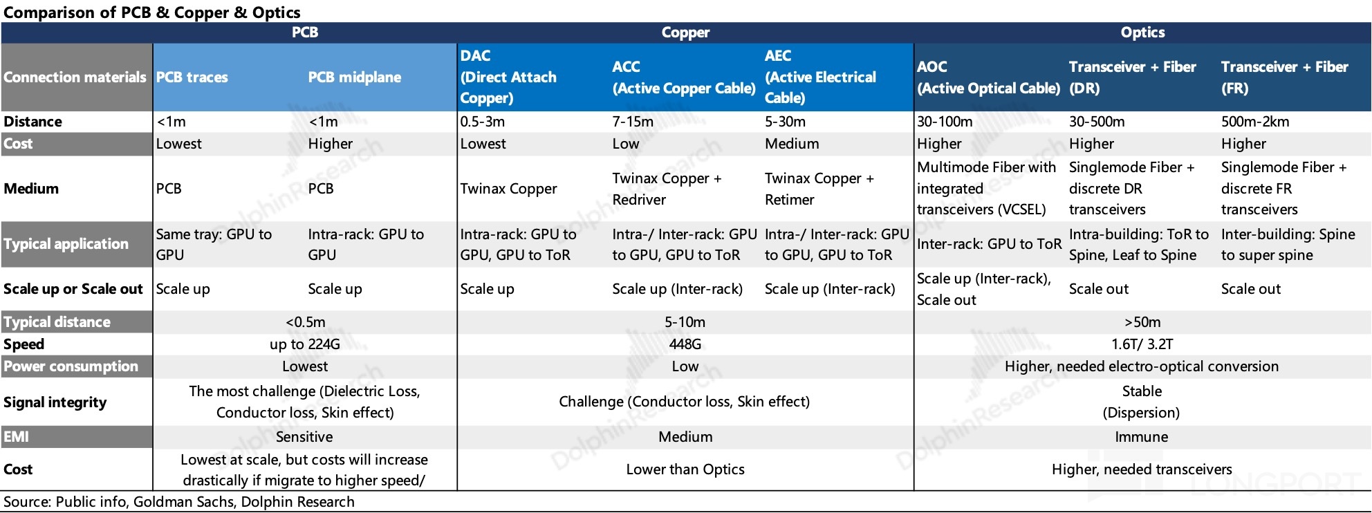
Copper has been favored for low power, cost efficiency, and reliability, but signal quality degrades quickly with distance and speed. Copper links are typically capped at ≤30 m, so copper is largely confined to in-cabinet Scale-Up. In Nvidia’s Rubin Ultra, PCB backplanes are introduced for in-cabinet Scale-Up for the first time, replacing copper cables.

Optical links offer high bandwidth and long reach with low loss, scale to Tbps, and thus dominate inter-rack links in Scale-Out.

c) NIC/DPU

The NIC is the network endpoint of a node, attached to xPUs/CPUs via PCIe or proprietary links, and sends/receives packets to switches. Its performance drives realized Scale-Out efficiency.

NICs are rapidly evolving into SmartNICs with onboard programmable logic, offloading non-core tasks from CPUs to free CPU cycles for AI orchestration. DPUs go further by taking over networking, storage, and security tasks.

2) How does the hardware operate?

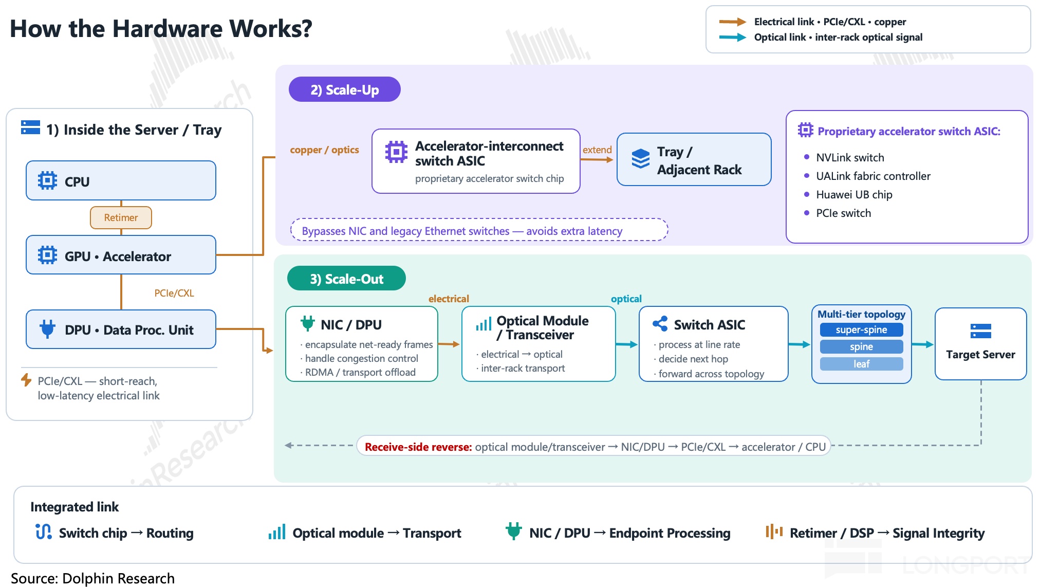
Each component has a defined role in the AI network. The next question is how they collaborate to execute AI workloads. We change perspective to trace the signal path and see how the pieces form a system.

See the overall flow below:

a) Within a node

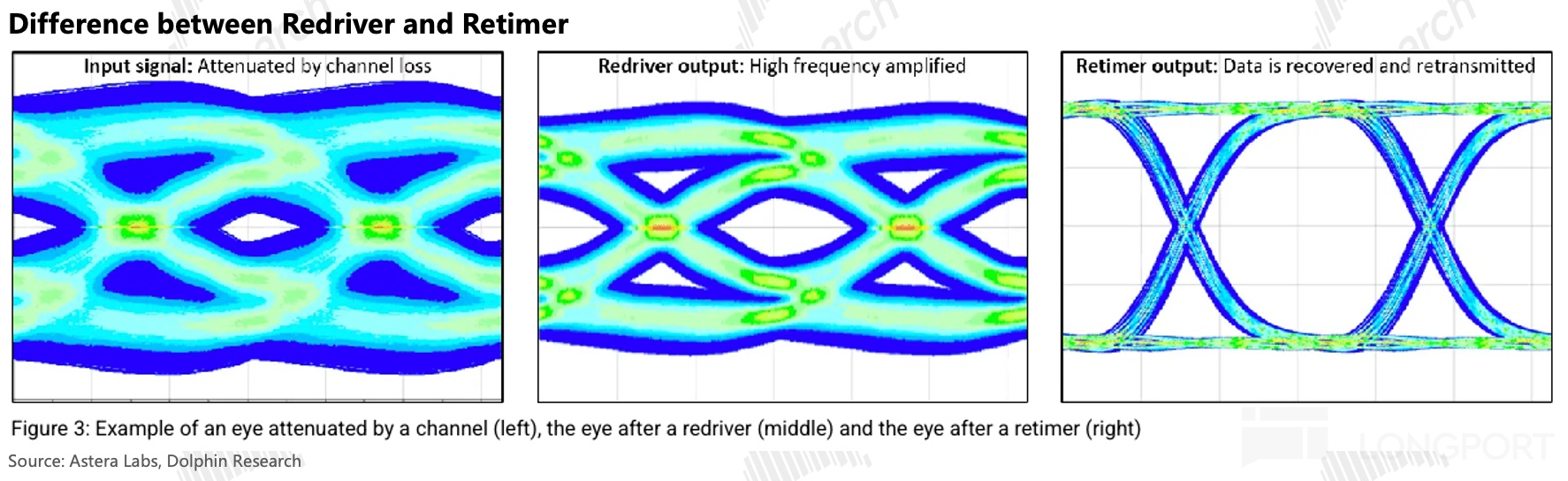
Inside a server, CPUs, GPUs, and NICs/DPUs are linked over electrical (copper) channels. When signal integrity cannot sustain the distance, redrivers and retimers are added.

Redrivers equalize and amplify in the analog domain, compensating high-frequency loss but also amplifying noise, at lower cost and power. Retimers re-time severely attenuated signals and retransmit so that downstream sees a brand-new link, extending reach.

b) Scale-Up

If the target accelerator is in the same domain, traffic goes through a proprietary interconnect switch ASIC (the office–dispatcher path), using load/store for direct addressing.

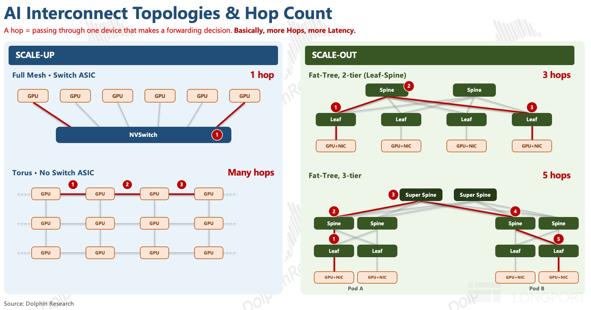
This introduces the common metric of hop count: each device that makes a forwarding decision adds one hop, and more hops mean higher latency.

With a switch ASIC in the Scale-Up domain, packets traverse a single ASIC hop to the destination GPU, so any GPU pair is one hop. Without a switch ASIC and using direct meshes (e.g., Torus — we will cover Google’s topology next time), similar scale requires multi-hop detours. Two-tier fat trees on Scale-Out take 3 hops; three-tier fat trees take 5 (see below).

These concepts are critical. First, place critical devices within the same communication semantic to allow direct addressing and speed. Second, minimize intermediate transfers — i.e., reduce hop count.

c) Scale-Out

If the target accelerator is outside the Scale-Up domain, traffic is handed to the NIC/DPU, then enters the optical module over an electrical channel. After E (electrical)/O (optical) conversion, it traverses fiber across racks.

At the switch, the optical module performs O/E, the switch ASIC processes the electrical signal, determines the next hop, and forwards. In multi-tier topologies, packets pass Leaf, Spine, then Super-Spine to reach the destination server.

III. The ecosystem battle: protocol is the soul

With hardware covered, we turn to protocols. If hardware is the infrastructure, protocols are the operating rules, defining communication semantics and the max scalable node count.

Latency and bandwidth needs vary widely by layer. Protocol ecosystems form competing camps whose strength depends on peer and supply-chain adoption of the standard, and on hardware shipments and share under that standard:

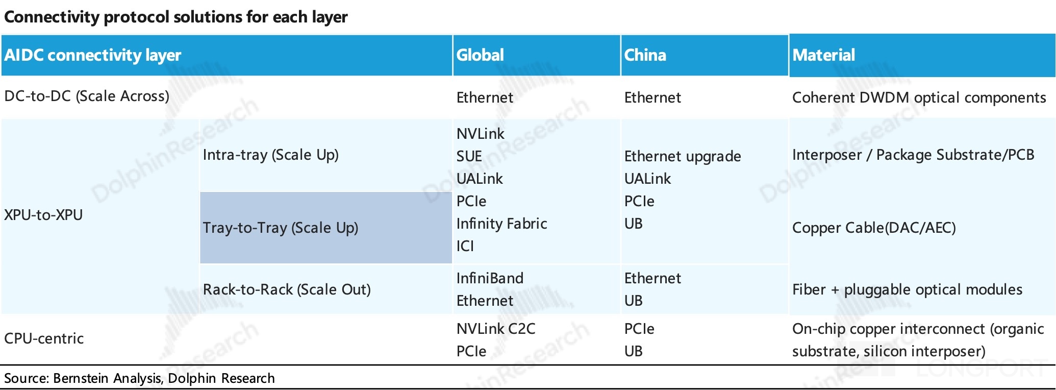
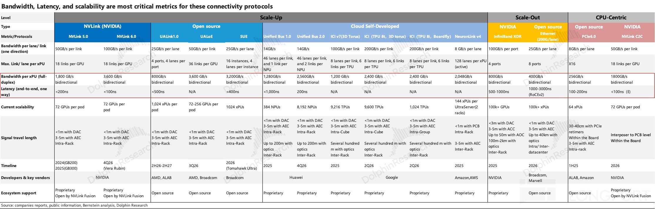
We summarize protocol performance by layer (see above), with bandwidth and latency as the key metrics (red boxes).

By layer, innovation concentrates in Scale-Up, where vendors seek to be the standard-setter, with proprietary protocols such as Nvidia NVLink, AMD UALink, and Huawei UB coexisting with different performance, cost, and ecosystem trade-offs.

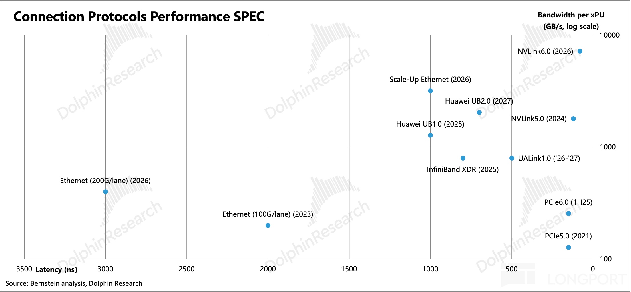
The Scale-Out landscape is clearer, with competition between Nvidia-led InfiniBand and Ethernet’s open ecosystem. On raw protocol performance, Nvidia still sets the bar and offers both closed and open-ecosystem options in parallel (the further up/right below, the better).

For CSPs, final choices balance workload needs, budgets, and control, enabling open camps like UALink and Broadcom SUE to form.

This primer on network connectivity stops here. Next we will compare AMD and Nvidia approaches to assess whether Helios can truly challenge Nvidia GB and VR NVL 72.

Related notes from Dolphin Research:

Jun 3, 2026: AI 超连接时代：AI 向 “光” 飞奔？

Jun 24, 2026: “‘铜’ 牛夫人” 不走！CPO：真机会 or 镜中花？

Risk disclosure and disclaimer: 海豚投研免责声明及一般披露